Dataframes classic intro
Let's check how counting words works for dataframes
scala> val rddTextFile=sc.textFile("LICENSE")

scala> rddTextFile.count
res1: Long = 953
Ok and now time for Dataframe
scala> val fileDF=rddTextFile.toDF("line")
fileDF: org.apache.spark.sql.DataFrame = [line: string]
We can check that we have a very sophisticated schema
scala> fileDF.printSchema
root
 |-- line: string (nullable = true)
And display soem content from DataFrame
scala> fileDF.show(10)
+--------------------+
|                line|
+--------------------+
|                    |
|                 ...|
|                 ...|
|                 ...|
|                    |
|   TERMS AND COND...|
|                    |
|     1. Definitions.|
|                    |
|      "License" s...|
+--------------------+
only showing top 10 rows
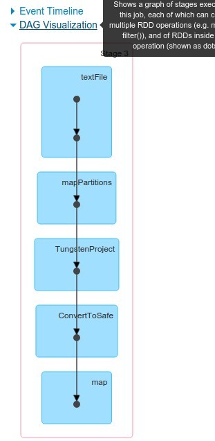
It's time to see how dataframes are represented in Web UI. We can see that mapping between what we do in REPL and what we see in UI is not as obvious as in case of RDDs. This is the price for higher abstraction.
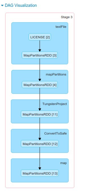
And let's see that after all everything is mapped to RDD
scala> val wordsDF=fileDF.explode("line","word"){(line:String) => line.split(" ")}
wordsDF: org.apache.spark.sql.DataFrame = [line: string, word: string]

//Or with some magic
scala> val wordsDF=fileDF.explode("line","word"){(_:String).split(" ")}
wordsDF: org.apache.spark.sql.DataFrame = [line: string, word: string]

scala> wordsDF.printSchema
root
 |-- line: string (nullable = true)
 |-- word: string (nullable = true)

scala> wordsDF.show(10)
+--------------------+----+
|                line|word|
+--------------------+----+
|                    |    |
|                 ...|    |
|                 ...|    |
|                 ...|    |
|                 ...|    |
|                 ...|    |
|                 ...|    |
|                 ...|    |
|                 ...|    |
|                 ...|    |
+--------------------+----+
only showing top 10 rows
For now results are not very exciting..
Column
This is actually an interesting moment when we are going outside simple "SQL table analogy". Look we can taka column from dataframe
scala> val wordCol=wordsDF("word")
wordCol: org.apache.spark.sql.Column = word
Now we can use columns in a function which carefully prepares domain filtering condition
scala> val condition=wordCol!==""
condition: org.apache.spark.sql.Column = NOT (word = )

scala> val notEmptyDF=wordsDF.select(wordCol).filter(condition)
notEmptyDF: org.apache.spark.sql.DataFrame = [word: string]

scala> notEmptyDF.show(10)
+--------------------+
|                word|
+--------------------+
|              Apache|
|             License|
|             Version|
|                2.0,|
|             January|
|                2004|
|http://www.apache...|
|               TERMS|
|                 AND|
|          CONDITIONS|
+--------------------+
only showing top 10 rows
That is a lot better!
Reduction
val result=wordsDF.filter($"word"!=="").groupBy($"word").count
scala> result.show(10)


+--------------------+-----+
|                word|count|
+--------------------+-----+
|          beneficial|    1|
|              ACTION|    5|
|               1995,|    2|
|                (now|    1|
|(net.sourceforge....|    1|
|              rights|   13|
|          derivative|   14|
|http://www.string...|    2|
|          litigation|    2|
|         conditions:|    5|
+--------------------+-----+

result.orderBy(result("count")).show(10)
+--------------------+-----+
|                word|count|
+--------------------+-----+
|           Pervasive|    1|
|             thereof|    1|
|               scopt|    1|
|           "License"|    1|
|            3-clause|    1|
|          BEOPEN.COM|    1|
|                (now|    1|
|          beneficial|    1|
|                (all|    1|
|(net.sourceforge....|    1|
+--------------------+-----+


// And finally
scala> result.orderBy(result("count").desc).show(10)
+----+-----+
|word|count|
+----+-----+
|   #|  279|
| the|  279|
|  of|  154|
|  to|  127|
| and|  126|
|  or|  124|
|  OR|  124|
|  OF|  102|
|  in|   89|
| THE|   69|
+----+-----+
only showing top 10 rows
Let's check UI to see what actually Happened.
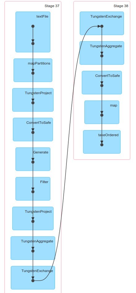
There is a lot of new things which we didn't saw when working with RDD. Let's take a closer look at the last phase.

So everything is mapped into RDDs but some are quite intersting ones like : "MapPartitionWithPreparationRDD". Catalyst optimizer in action.
https://databricks.com/blog/2015/04/13/deep-dive-into-spark-sqls-catalyst-optimizer.html
Ok, now we need to filter out stop words.
UDFs
scala> val stopWords=Set("#","the","of","to","and","or","in","the")
Let's now create a function to filter stop words
scala> val notStopWord:String=>Boolean = s=> !stopWords.contains(s)
notStopWord: String => Boolean = <function1>

scala> notStopWord("of")
res59: Boolean = false

scala> notStopWord("szczebrzeszyn")
res60: Boolean = true
Is using stop words in function a good Idea or should we somehow send this set to workers before calling lambdas?
Important Note - It is a FUNCTION! Not a stored procedure but a function which is easy to test and compose!!! End of important note
Let's register (or lift - for FP fans) our function to use columns level.
scala> val notStopWordUDF=sqlContext.udf.register("notStopWord",notStopWord)
notStopWordUDF: org.apache.spark.sql.UserDefinedFunction = UserDefinedFunction(<function1>,BooleanType,List())
And now time for a Combo
notEmptyDF.filter(notStopWordUDF(wordCol)).groupBy(wordCol).count.orderBy($"count".desc).show(10)
During workshops we will discuss why this line works. And the result is almost good.
+-------+-----+
|   word|count|
+-------+-----+
|     OR|  124|
|     OF|  102|
|    THE|   69|
|   this|   63|
|    ANY|   61|
|    any|   50|
|      a|   49|
|License|   45|
|   that|   44|
|      -|   44|
+-------+-----+
We can also use predefined function "lower" which oeprates on dataframe column.
scala> notEmptyDF.select(lower(wordCol).alias("word")).filter(notStopWordUDF($"word")).groupBy($"word").count.orderBy($"count".desc).show(10)
+---------+-----+
|     word|count|
+---------+-----+
|      any|  111|
|     this|   94|
|      for|   86|
|copyright|   65|
|  license|   64|
|        a|   64|
| software|   56|
|      not|   50|
|       by|   49|
|       is|   48|
+---------+-----+
only showing top 10 rows
Composition
If don't want to lower each word in file then we can compose function "lower" with our predefined function. But there is one problem : "lower" has type :
scala> lower _
res84: org.apache.spark.sql.Column => org.apache.spark.sql.Column = <function1>
And our defined function is actially a case class which needs to be converted into function
scala> notStopWordUDF.apply _
res86: Seq[org.apache.spark.sql.Column] => org.apache.spark.sql.Column = <function1>
And we have another problem because our function expectects sequence of Columns (varargs in apply). So to compose those two operations we need to create "glue lambda" (I don't know how to call it in other words)
val removeStopWords=(lower _) andThen (c=>notStopWordUDF.apply(c))

scala> notEmptyDF.filter(removeStopWords($"word").alias("word")).groupBy($"word").count.orderBy($"count".desc).show(10)
+-------+-----+
|   word|count|
+-------+-----+
|   this|   63|
|    ANY|   61|
|    any|   50|
|      a|   49|
|License|   45|
|   that|   44|
|      -|   44|
|    PSF|   38|
|     is|   37|
|     by|   36|
We can see that results are slightly different because we haven't converted every word to lower.
Full Program
sc.textFile("LICENSE").toDF("line")
.explode("line","word"){(line:String) => line.split("")}
.filter($"word"!=="").filter(removeStopWords($"word").alias("word"))
.groupBy($"word").count.orderBy($"count".desc).show(10)
+-------+-----+
|   word|count|
+-------+-----+
|   this|   63|
|    ANY|   61|
|    any|   50|
|      a|   49|
|License|   45|
|   that|   44|
|      -|   44|
|    PSF|   38|
|     is|   37|
|     by|   36|
+-------+-----+
And we arew orking on a level of abstraction which don't use words like map or flatMap.
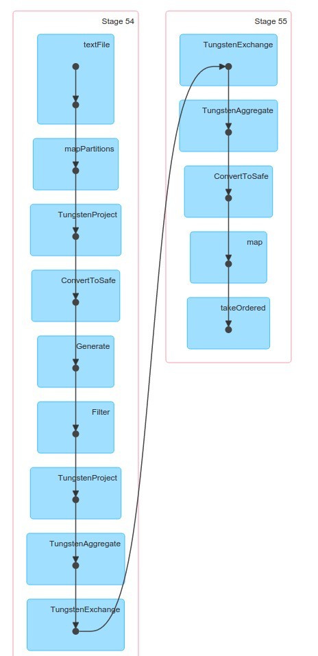
We can also check Details for SQL
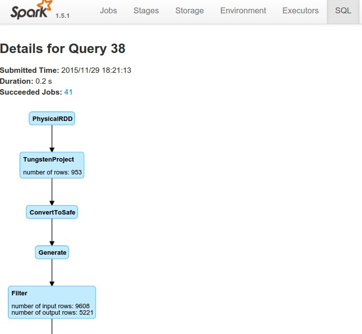
and also go in details through optimalization phases for our operations
== Parsed Logical Plan ==
Limit 11
 Sort [count#96L DESC], true
  Aggregate [word#94], [word#94,count(1) AS count#96L]
   Filter UDF(lower(word#94))
    Filter NOT (word#94 = )
     Generate UserDefinedGenerator(line#92), true, false, None, [word#94]
      Project [_1#91 AS line#92]
       LogicalRDD [_1#91], MapPartitionsRDD[283] at stringRddToDataFrameHolder at <console>:30

== Analyzed Logical Plan ==
word: string, count: bigint
Limit 11
 Sort [count#96L DESC], true
  Aggregate [word#94], [word#94,count(1) AS count#96L]
   Filter UDF(lower(word#94))
    Filter NOT (word#94 = )
     Generate UserDefinedGenerator(line#92), true, false, None, [word#94]
      Project [_1#91 AS line#92]
       LogicalRDD [_1#91], MapPartitionsRDD[283] at stringRddToDataFrameHolder at <console>:30

== Optimized Logical Plan ==
Limit 11
 Sort [count#96L DESC], true
  Aggregate [word#94], [word#94,count(1) AS count#96L]
   Project [word#94]
    Filter (NOT (word#94 = ) && UDF(lower(word#94)))
     Generate UserDefinedGenerator(line#92), true, false, None, [word#94]
      Project [_1#91 AS line#92]
       LogicalRDD [_1#91], MapPartitionsRDD[283] at stringRddToDataFrameHolder at <console>:30

== Physical Plan ==
TakeOrderedAndProject(limit=11, orderBy=[count#96L DESC], output=[word#94,count#96L])
 ConvertToSafe
  TungstenAggregate(key=[word#94], functions=[(count(1),mode=Final,isDistinct=false)], output=[word#94,count#96L])
   TungstenExchange hashpartitioning(word#94)
    TungstenAggregate(key=[word#94], functions=[(count(1),mode=Partial,isDistinct=false)], output=[word#94,currentCount#99L])
     TungstenProject [word#94]
      Filter (NOT (word#94 = ) && UDF(lower(word#94)))
       !Generate UserDefinedGenerator(line#92), true, false, [line#92,word#94]
        ConvertToSafe
         TungstenProject [_1#91 AS line#92]
          Scan PhysicalRDD[_1#91]

Code Generation: true
Read CSV
We need to start Spark like this :
bin/spark-shell --packages com.databricks:spark-csv_2.10:1.3.0
So it will automatically download csv plugin.
val plDF=sqlContext.read.format("com.databricks.spark.csv").option("header", "true").option("inferSchema", "true").load("E0.csv"
This is what we will use : http://www.football-data.co.uk/mmz4281/1415/E0.csv
and here is column description: http://www.football-data.co.uk/notes.txt
And we can see quite big schema
scala> plDF.printSchema
root
 |-- Div: string (nullable = true)
 |-- Date: string (nullable = true)
 |-- HomeTeam: string (nullable = true)
 |-- AwayTeam: string (nullable = true)
 |-- FTHG: integer (nullable = true)
 |-- FTAG: integer (nullable = true)
 |-- FTR: string (nullable = true)
 |-- HTHG: integer (nullable = true)
 |-- HTAG: integer (nullable = true)
 |-- HTR: string (nullable = true)
 |-- Referee: string (nullable = true)
 |-- HS: integer (nullable = true)
 |-- AS: integer (nullable = true)
 |-- HST: integer (nullable = true)
(...and more...)
Full SQL
Now let's see soemthign else. We can actually map dataframe to notmal sql by registering temp table
scala> plDF.registerTempTable("premierleague")

val footFrame=sqlContext.sql ("select HomeTeam as team,HS as shoots ,HST shoots_target from premierleague")
footFrame: org.apache.spark.sql.DataFrame = [team: string, shoots: int, shoots_target: int]

scala> footFrame.show(10)
+----------+------+-------------+
|      team|shoots|shoots_target|
+----------+------+-------------+
|   Arsenal|    14|            6|
| Leicester|    11|            3|
|Man United|    14|            5|
|       QPR|    19|            6|
|     Stoke|    12|            2|
| West Brom|    10|            5|
|  West Ham|    18|            4|
| Liverpool|    12|            5|
| Newcastle|    12|            0|
|   Burnley|     9|            2|
+----------+------+-------------+
Now let's create UDF which counts percentage of shots on target
scala> val accuracy : (Int,Int) => Double = (shootsTarget,shoots) => (shootsTarget.toDouble/ shoots.toDouble)*100
accuracy: (Int, Int) => Double = <function2>

//We can use easily scalacheck here
scala> accuracy(5,10)
res9: Double = 50.0

scala> accuracy(3,20)
res10: Double = 15.0

scala> accuracy(7,20)
res11: Double = 35.0
Lift pure fucntion to column
scala> val accuracyUDF =udf(accuracy)
accuracyUDF: org.apache.spark.sql.UserDefinedFunction = UserDefinedFunction(<function2>,DoubleType,List(IntegerType, IntegerType))
Add Accuracy column
scala> val accFrame =footFrame.withColumn("accuracy",accuracyUDF($"shoots_target",$"shoots"))
accFrame: org.apache.spark.sql.DataFrame = [team: string, shoots: int, shoots_target: int, accuracy: double]

scala> accFrame.show(10)
+----------+------+-------------+------------------+
|      team|shoots|shoots_target|          accuracy|
+----------+------+-------------+------------------+
|   Arsenal|    14|            6|42.857142857142854|
| Leicester|    11|            3| 27.27272727272727|
|Man United|    14|            5|35.714285714285715|
|       QPR|    19|            6| 31.57894736842105|
|     Stoke|    12|            2|16.666666666666664|
| West Brom|    10|            5|              50.0|
|  West Ham|    18|            4| 22.22222222222222|
| Liverpool|    12|            5| 41.66666666666667|
| Newcastle|    12|            0|               0.0|
|   Burnley|     9|            2| 22.22222222222222|
+----------+------+-------------+------------------+
Now some serious Data Science!!
Ten the most accurate teams in 2014
scala> accFrame.groupBy($"team").agg(avg("accuracy").alias("avgAcc")).orderBy($"avgAcc".desc).show(10)
+--------------+------------------+
|          team|            avgAcc|
+--------------+------------------+
|       Chelsea| 41.98844127382444|
|       Arsenal| 39.17117668688947|
|    Man United|37.850357151513364|
|       Swansea| 36.67447241893226|
|      Man City|35.149588998836165|
|   Southampton|34.675709091582874|
|Crystal Palace|34.149016165881086|
|     West Brom| 33.04894986110493|
|          Hull|  32.4177945784594|
|       Everton| 31.75502043536099|
+--------------+------------------+
only showing top 10 rows
Ten the least accurate teams in 2014
scala> accFrame.groupBy($"team").agg(avg("accuracy").alias("avgAcc")).orderBy($"avgAcc".asc).show(10)
+-----------+------------------+
|       team|            avgAcc|
+-----------+------------------+
|      Stoke| 25.31579664558531|
| Sunderland|26.755766163660898|
|Aston Villa| 28.98439280018227|
|  Leicester|30.022138526293656|
|  Newcastle| 30.67953658873489|
|        QPR| 30.79045800306188|
|  Liverpool|  31.4443402420427|
|  Tottenham|31.506379478246483|
|   West Ham|31.648911477832154|
|    Burnley|31.745868510574393|
+-----------+------------------+
Read from Hive -
To show that Spark is not living outside big data world it should be interesting to show how it cooperates with Hive.
To do it let's use recent Cloudera QuickStart VM 5.5 which has Spark version 1.5.0
http://www.cloudera.com/content/www/en-us/downloads/quickstart_vms/5-5.html
Then you need to perform first exercise during which you are going to import data from mysql to hive with sqoop
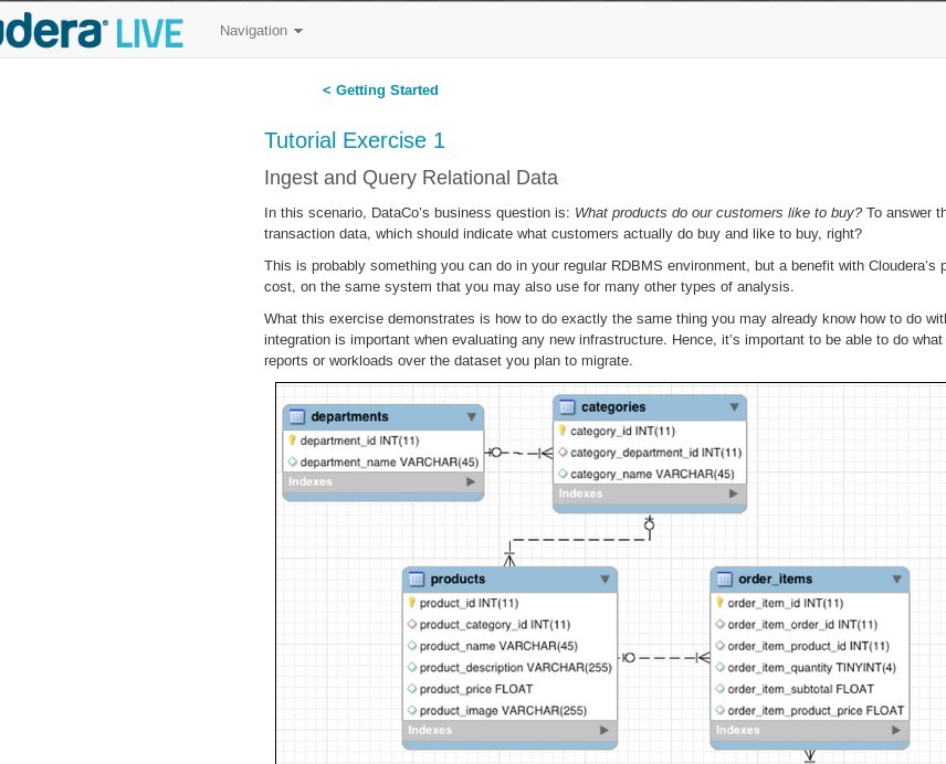
Now Let's copy hive config to spark config folder to allow spark read hive tables.
[cloudera@quickstart spark]$ sudo cp /etc/hive/conf/hive-site.xml /etc/spark/conf/hive-site.xml
And we can play
val customersDF=sqlContext.sql("select customer_id,customer_fname,customer_lname from customers")

scala> customersDF.printSchema
root
 |-- customer_id: integer (nullable = true)
 |-- customer_fname: string (nullable = true)
 |-- customer_lname: string (nullable = true)


scala> val ordersDF=sqlContext.sql("select order_id,order_customer_id from orders where order_status = 'COMPLETE' ")
ordersDF: org.apache.spark.sql.DataFrame = [order_id: int, order_customer_id: int]

scala> ordersDF.printSchema
root
 |-- order_id: integer (nullable = true)
 |-- order_customer_id: integer (nullable = true)
Let's do a simple join
scala> val joined=customersDF.join(ordersDF,$"customer_id" === $"order_customer_id")
joined: org.apache.spark.sql.DataFrame = [customer_id: int, customer_fname: string, customer_lname: string, order_id: int, order_customer_id: int]

scala> joined.printSchema
root
 |-- customer_id: integer (nullable = true)
 |-- customer_fname: string (nullable = true)
 |-- customer_lname: string (nullable = true)
 |-- order_id: integer (nullable = true)
 |-- order_customer_id: integer (nullable = true)
And DATASCIENCE!!!
Top 10 customers
scala> joined.groupBy($"customer_lname",$"customer_fname").count.orderBy($"count".desc).show(10)
+--------------+--------------+-----+
|customer_lname|customer_fname|count|
+--------------+--------------+-----+
|         Smith|          Mary| 3153|
|         Smith|        Robert|   99|
|         Smith|         James|   95|
|         Smith|          John|   86|
|         Smith|         David|   82|
|         Smith|       William|   66|
|         Jones|          Mary|   64|
|         Smith|       Michael|   62|
|         Smith|       Matthew|   50|
|         Smith|   Christopher|   49|
+--------------+--------------+-----+
only showing top 10 rows
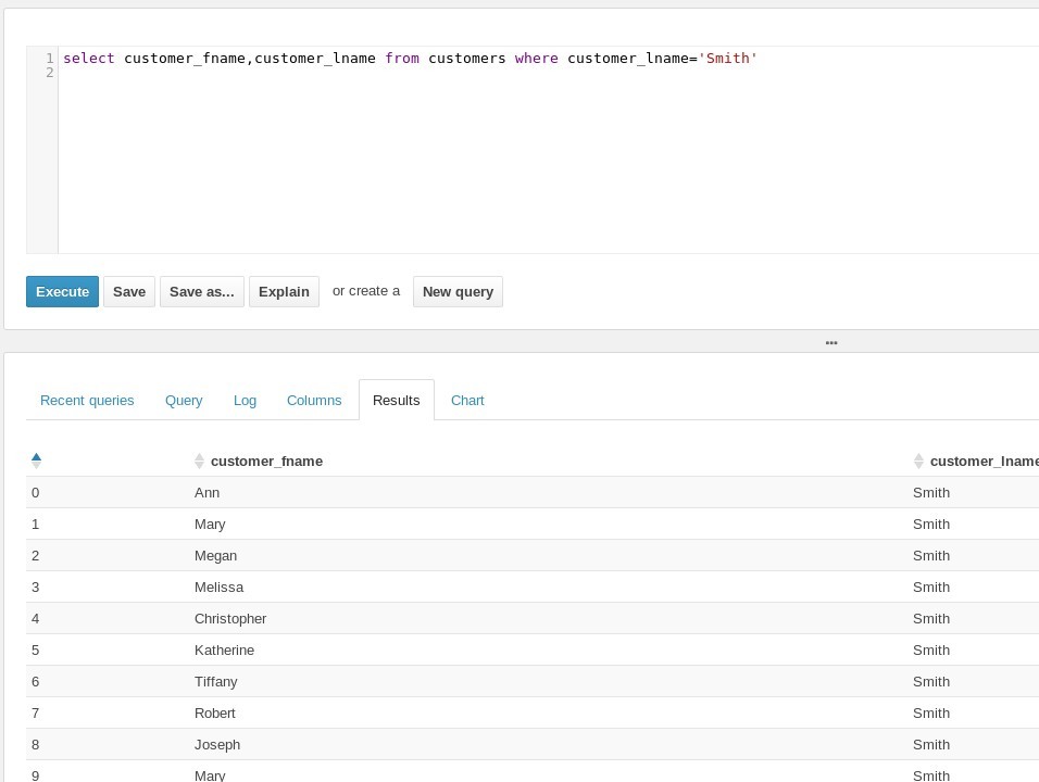
Indeed there is a big gang of Smiths in the Hive
SparkR
As the last exercise we can look a little bit closer at SparkR and R language from where Dataframes concepts was borrowed
First of all we need to have R language installed and then we can start SparkR
~/bin/Spark$ bin/sparkR

R version 3.2.2 (2015-08-14) -- "Fire Safety"
Copyright (C) 2015 The R Foundation for Statistical Computing
Platform: x86_64-pc-linux-gnu (64-bit)
R has and example dataframe called mtcars which we will use for this tutorial
> mtcars
                     mpg cyl  disp  hp drat    wt  qsec vs am gear carb
Mazda RX4           21.0   6 160.0 110 3.90 2.620 16.46  0  1    4    4
Mazda RX4 Wag       21.0   6 160.0 110 3.90 2.875 17.02  0  1    4    4
Datsun 710          22.8   4 108.0  93 3.85 2.320 18.61  1  1    4    1
Hornet 4 Drive      21.4   6 258.0 110 3.08 3.215 19.44  1  0    3    1
Hornet Sportabout   18.7   8 360.0 175 3.15 3.440 17.02  0  0    3    2
Valiant             18.1   6 225.0 105 2.76 3.460 20.22  1  0    3    1
Duster 360          14.3   8 360.0 245 3.21 3.570 15.84  0  0    3    4
Merc 240D           24.4   4 146.7  62 3.69 3.190 20.00  1  0    4    2
Merc 230            22.8   4 140.8  95 3.92 3.150 22.90  1  0    4    2
Merc 280            19.2   6 167.6 123 3.92 3.440 18.30  1  0    4    4
Merc 280C           17.8   6 167.6 123 3.92 3.440 18.90  1  0    4    4
Let's create SparkR dataframe from R dataframe - first attempt
> sparkCars <- createDataFrame(sqlContext, mtcars)
> sparkCars
DataFrame[mpg:double, cyl:double, disp:double, hp:double, drat:double, wt:double, qsec:double, vs:double, am:double, gear:double, carb:double]
> head(sparkCars)
   mpg cyl disp  hp drat    wt  qsec vs am gear carb
1 21.0   6  160 110 3.90 2.620 16.46  0  1    4    4
2 21.0   6  160 110 3.90 2.875 17.02  0  1    4    4
3 22.8   4  108  93 3.85 2.320 18.61  1  1    4    1
4 21.4   6  258 110 3.08 3.215 19.44  1  0    3    1
5 18.7   8  360 175 3.15 3.440 17.02  0  0    3    2
6 18.1   6  225 105 2.76 3.460 20.22  1  0    3    1
We don't have column names so let's try it again
> carNames<-rownames(mtcars)
> carNames
 [1] "Mazda RX4"           "Mazda RX4 Wag"       "Datsun 710"
 [4] "Hornet 4 Drive"      "Hornet Sportabout"   "Valiant"
 [7] "Duster 360"          "Merc 240D"           "Merc 230"
[10] "Merc 280"            "Merc 280C"           "Merc 450SE"
[13] "Merc 450SL"          "Merc 450SLC"         "Cadillac Fleetwood"
[16] "Lincoln Continental" "Chrysler Imperial"   "Fiat 128"
[19] "Honda Civic"         "Toyota Corolla"      "Toyota Corona"
[22] "Dodge Challenger"    "AMC Javelin"         "Camaro Z28"
[25] "Pontiac Firebird"    "Fiat X1-9"           "Porsche 914-2"
[28] "Lotus Europa"        "Ford Pantera L"      "Ferrari Dino"
[31] "Maserati Bora"       "Volvo 142E"
> frameWithNames<-cbind(carNames,mtcars)
> sparkCars<-createDataFrame(sqlContext,frameWithNames)
> head(sparkCars)
           carNames  mpg cyl disp  hp drat    wt  qsec vs am gear carb
1         Mazda RX4 21.0   6  160 110 3.90 2.620 16.46  0  1    4    4
2     Mazda RX4 Wag 21.0   6  160 110 3.90 2.875 17.02  0  1    4    4
3        Datsun 710 22.8   4  108  93 3.85 2.320 18.61  1  1    4    1
4    Hornet 4 Drive 21.4   6  258 110 3.08 3.215 19.44  1  0    3    1
5 Hornet Sportabout 18.7   8  360 175 3.15 3.440 17.02  0  0    3    2
6           Valiant 18.1   6  225 105 2.76 3.460 20.22  1  0    3    1
Now let's filter out all cars which have less or 6 cylinders.
> bigEngine<-sparkCars[sparkCars$cyl > 6]
> head(bigEngine)
            carNames  mpg cyl  disp  hp drat   wt  qsec vs am gear carb
1  Hornet Sportabout 18.7   8 360.0 175 3.15 3.44 17.02  0  0    3    2
2         Duster 360 14.3   8 360.0 245 3.21 3.57 15.84  0  0    3    4
3         Merc 450SE 16.4   8 275.8 180 3.07 4.07 17.40  0  0    3    3
4         Merc 450SL 17.3   8 275.8 180 3.07 3.73 17.60  0  0    3    3
5        Merc 450SLC 15.2   8 275.8 180 3.07 3.78 18.00  0  0    3    3
6 Cadillac Fleetwood 10.4   8 472.0 205 2.93 5.25 17.98  0  0    3    4
And finally we will take a hp column and calculate average speed of those cars
> mhp <- mean(bigEngine$hp)
> mhp
Column avg(hp)
> showDF(select(bigEngine,mhp))
+------------------+
|           avg(hp)|
+------------------+
|209.21428571428572|
+------------------+
And this should be more than enough for an interesting introduction to DataFrames in Spark!
links
https://databricks.com/blog/2015/08/12/from-pandas-to-apache-sparks-dataframe.html https://ogirardot.wordpress.com/2015/05/29/rdds-are-the-new-bytecode-of-apache-spark/ https://www.mapr.com/ebooks/spark/chapter05-processing-tabular-data.html http://www.nodalpoint.com/dataframes-from-csv-files-in-spark-1-5-automatic-schema-extraction-neat-summary-statistics-elementary-data-exploration/ http://www.nodalpoint.com/spark-data-frames-from-csv-files-handling-headers-column-types/ https://databricks.com/blog/2015/02/17/introducing-dataframes-in-spark-for-large-scale-data-science.html https://dzone.com/articles/using-apache-spark-dataframes-for-processing-of-ta http://blog.knoldus.com/2015/10/21/using-spark-dataframes-for-word-count/